Identifying Air Pollution Data Manipulation in China

Introduction

In 2010, air pollution levels in Beijing exceeded the bounds of the EPA’s air quality index, leading the U.S. Embassy to deem the city’s air quality “crazy bad”. Although China’s work in building a national system of air pollution standards dates back to 1982, enforcement of the standards – particularly at the local level – has been difficult. In an attempt to encourage enforcement and investment in air quality improvements, the government began in 1989 to include compliance with environmental standards into performance evaluations of local government officials.

As these evaluations were part of the cadre promotion system in China, the intent was to incentivize local officials to take concrete steps towards improving local air quality. Points were awarded to cities based on their annual percentage of blue-sky days – those days with a local air pollution index (API) below 100. However, given that the data on air quality were largely self-reported by local governments, the opportunities and incentives for officials to manipulate their reported data were significant.

Such misinformation can produce large social costs. Studies have shown, for example, that public alert systems work well in encouraging people to reduce outdoor activities when air quality is particularly bad, which can significantly reduce the adverse health impacts of air pollution. However, issuing alerts is typically contingent upon reaching certain levels of pollution. Additionally, being able to manipulate data can reduce the pressure on local officials to adopt actual measures to improve air quality.

Methods

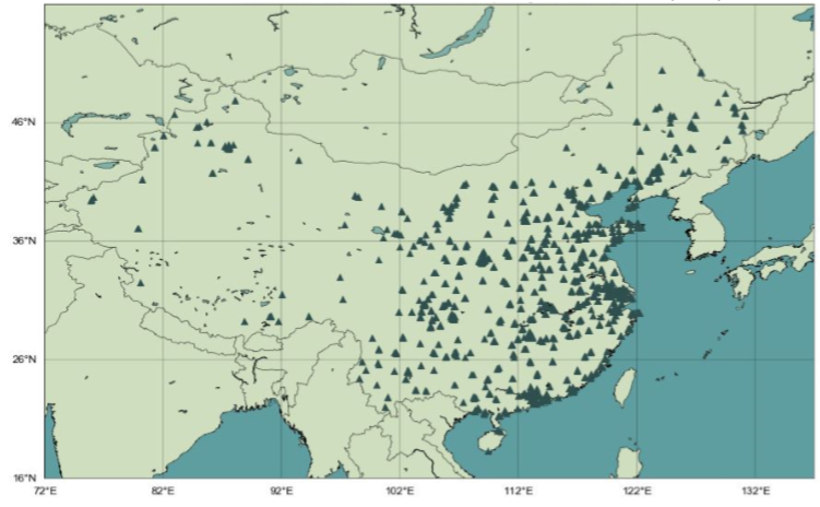
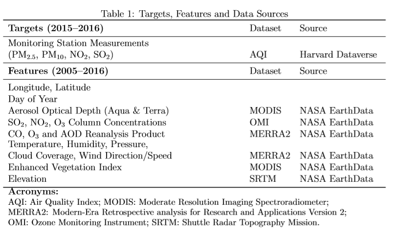
Using machine learning techniques and a rich dataset of satellite images from NASA, we reconstructed historical air pollution levels to compare to officially reported data, with the goal of identifying localities where the manipulation of air pollution data (i.e. API) may have occurred. We accomplished this by training a model with reliable pollution data for 2015 to 2016, to reconstruct levels for the same pollutants from 2005 to 2014 for all monitoring stations in the country, the locations of which are depicted in the figure below. The table following the figure shows all the features used in our dataset and a list of our target variables.

The targets (monitoring station measurements for four pollutants from 2015-2016) are considered to be reliable, because they are sourced from stations that automatically report real-time data, publicized on data-center websites. Using the features listed above, we train and test a model on the 2015 and 2016 data, and then use it to predict levels of PM10, NO2, and SO2 across monitoring stations for 2005-2014.

All the input datasets are satellite images with values recorded on regular grids. We first match them with coordinates of the monitoring stations and extract values corresponding to the specific stations. To include relevant spatial and temporal information, we also apply an Epanechnikov kernel with a spatial bandwidth of 1.5 degree (the approximate distance over which air pollutants can travel in one day), discard missing values, and extract a variable of the reweighted mean of all the values within the bandwidth of the kernel. Three-day and seven-day moving averages of some variables are also added to the model to reduce the number of missing values.

Unlike previous papers, instead of training a model for all the stations in our dataset, we train a separate model for every single monitoring station in our sample. This takes into account the possibility that the data generating process in different stations may be different in nature (e.g. in high altitudes, chemical reactions follow a different pattern than places in low altitudes) and leverages the fact that our training data is sufficiently large to allow for this. We used several machine learning algorithms for regression, including random forest, multi-layer perceptron (MLP), gradient boosting machine, and extreme gradient boosting. After feature engineering and tuning, the best performing algorithms were gradient boosting and extreme gradient boosting machine, the latter of which yielded a median R2 of around 50%. Table 2 below provides a summary of the performance for these top two algorithms.

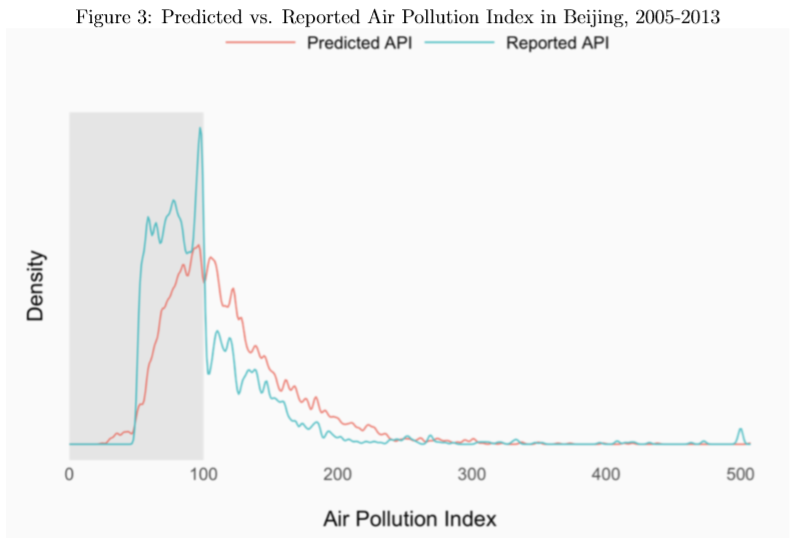
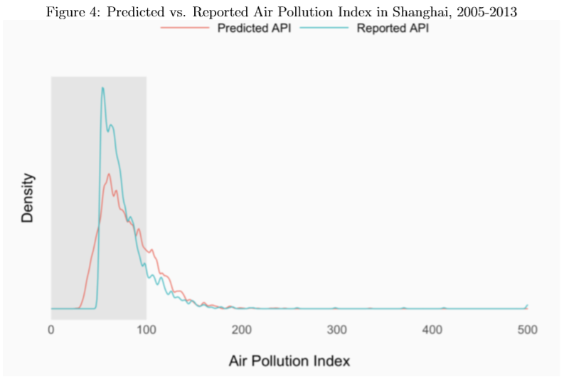
As PM10, SO2, and NO2 are the only pollution variables included in calculating the Air Pollution Index (API) before 2013 (a year after which the calculation of API was amended), we use our predictions of these variables to calculate – per the formulation of API in the existing literature – predicted API scores over 2005 to 2013, and compare these predicted values to the officially reported API values over the same time period. These comparisons are shown for Beijing and Shanghai in the following two figures. The density of officially reported API scores for Beijing has a clear discontinuity just below the threshold level of API=100, whereas the density of our predicted API for Beijing shows a skewed, but otherwise well-behaved probability distribution. The lack of a discontinuity in the distribution of our predicted values provides some evidence for assessing the potential manipulation of the official API scores in the past for Beijing.

In contrast, for Shanghai, we do not observe such a discontinuity in the officially reported API values over the same period (2005-2013), which suggests that data manipulation of reported API may not have occurred for officials in Shanghai.

Considering government-reported API values before the advent of automatic reporting at monitoring stations (i.e. pre-2015 in our data), as well as our predicted distributions of API values over the same time period and by monitoring station, we also use Welch’s t-tests to assess whether the predicted and reported API values have equal means, an approach which provides another measure by which to identify potential data manipulators.

Additional Considerations

Because we only have training data for 2015-2016, but apply our model out-of-sample to predict pollutant levels for 2005-2014, a concern in this project is that the underlying data generating process may experience temporal variation that our model can not capture. For example, changes in the composition of air pollutants may shift, which may then change the functional relationships that we are trying to model. Future work should thus address potential time inconsistency issues around the data generating process.